The Training Sets

Next: The Algorithm Up: Modeling Previous: Modeling

The Training Sets

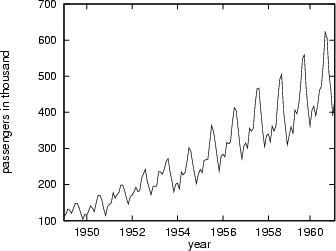
As test bed for our forecasting system we used two well known time series from [BJ76]: The monthly totals of international airline passengers (thousand of passengers) from 1949 to 1960 (see figure 4), and the daily closing prices of IBM common stock from May 1961 to November 1962 (see figure 5).

**Figure 4:** International airline passengers
$\begin{figure} \centerline{ \epsfbox {airlinepass.eps} }\end{figure}$

**Figure 5:** IBM share price
$\begin{figure} \centerline{ \epsfbox {ibmshares.eps} }\end{figure}$

Table 1 gives some characteristics of these two time series: $\sigma$ is the standard deviation, $\mu$ the mean, and n the number of observations. The airline time series is an example of time series data with a clear trend and multiplicative seasonality, whereas the IBM share price shows a break in the last third of the series and no obvious trend and/or seasonality.

**Figure:** Properties of time series
$\begin{figure} \leavevmode \begin{center} \begin{tabular} {\vert l\vert r\ver... ...ngers & 119.55 & 280.30 & 144 \\ \hline \end{tabular} \end{center}\end{figure}$

The next section is concerned with the question: How can a neural network learn a time series?