Network Parameters

The following parameters of the artificial neural network were chosen for a closer inspection:

• The learning rate $\eta$

  $\eta$ ($0<\eta<1$) is a scaling factor that tells the learning algorithm how strong the weights of the connections should be adjusted for a given error. A higher $\eta$ can be used to speed up the learning process, but if $\eta$ is too high, the algorithm will ``step over'' the optimum weights. The learning rate $\eta$ is constant across presentations.

• The momentum $\alpha$

  The momentum parameter $\alpha$ ($0<\alpha<1$) is another number that affects the gradient descent of the weights: To prevent each connection from following every little change in the solution space immediately, the momentum term is added that keeps the direction of the previous step [HKP91], thus avoiding the descent into local minima. The momentum term is constant across presentations.

• The number of input and the number of hidden units (the network topology).

  The number of input units determines the number of periods the neural network ``looks into the past'' when predicting the future. The number of input units is equivalent to the size of the input window.

  Whereas it has been shown that one hidden layer is sufficient to approximate continuous function [HSW89], the number of hidden units necessary is ``not known in general [HKP91]''. Other approaches for time series analysis with artificial neural networks report working network topologies (number of neurons in the input-hidden-output layer) of 8-8-1, 6-6-1 [CMMR92], and 5-5-1 [Whi88].

To examine the distribution of these parameters, we conducted a number of experiments: In subsequent runs of the network, these parameters were systematically changed to explore their effect on the network's modeling and forecasting capabilities.

We used the following terms to measure the modeling quality s_m and forecasting quality s_f of our system: For a time series $X_1,\ldots,X_n$ 

$$s_m = \sqrt{\frac{\sum\limits_{i=1}^n(X_i-\hat{X}_i)^2}{n}}$$ (1)

 

$$s_f = \sqrt{\frac{\sum\limits_{i=n+1}^{n+1+r}(X_i-\hat{X}_i)^2}{r}}$$ (2)

where $\hat{X}_i$ is the estimate of the artificial neural network for period i and r is the number of forecasting periods. The error s_m (equation 1) estimates the capability of the neural network to mimic the known data set, the error s_f (equation 2) judges the networks's forecast capability for a forecast period of length r. In our experiments, we used r=20.

Note: For reasons of clarity, in this section we only present graphics for the IBM share price time series. The graphics for the airline passenger time series are very similar.

The figures 7 and 8 demonstrate the effect of variations of the learning rate $\eta$and the momentum $\alpha$ on the modeling (figure 7) and forecast (figure 8) quality: both graphics give evidence for the robustness of the backpropagation algorithm, high values of both $\eta$ and $\alpha$ should be avoided.

  

Figure: Learning rate and momentum, IBM share price, modeling quality

  

Figure: Learning rate and momentum, IBM share price, forecasting quality

The figures 10 and 11 present the effect of different network topologies on the modeling (figure 10) and forecasting (figure 11) quality: The number of input units and the number of hidden units open an interesting view: artificial neural networks with more than approx. 50 hidden units are not suited for the task of time series forecasting. This tendency of ``over-elaborate networks capable of data-miming'' is also reported by [Whi88].

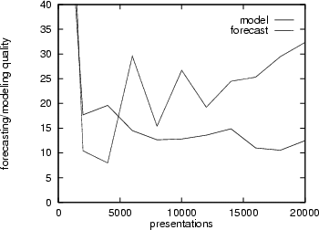
Another parameter we have to consider is the number of presentations. A longer training period does not necessarily result in a better forecasting capability. Figure 9 demonstrates this ``overlearning'' effect for the IBM share price time series: with an increasing number of presentations, the network memorizes details of the time series data instead of learning its essential features. This loss of generalization power has a negative effect on the network's forecasting ability.

  

Figure 9: Modeling vs. forecasting ability

These estimations of the network's most important parameters, although rough, allowed us to choose reasonable parameters for our performance comparison with the ARIMA technique, described in the next section.

  

Figure: Number of input and hidden units, IBM share price, modeling quality

  

Figure: Number of input and hidden units, IBM share price, forecasting quality