Gottfried Rudorfer, Early Bankruptcy Detection Using Neural Networks,
APL Quote Quad, ACM New York, Volume 25, Number 4, June 1995, pages 171-178
Early Bankruptcy Detection Using Neural Networks
Gottfried Rudorfer
Department of Applied Computer Science
University of Economics and Business Administration
Augasse 2-6
A-1090 Vienna
Austria
This email address is being protected from spambots. You need JavaScript enabled to view it.
Download the PDF-version here.
Abstract
In 1993, Austria had the highest number of bankruptcies since 1945. The total liabilities came to approx. US$ 3 Billion.
Powerful tools for early detection of company risks are very important to avoid high economic losses. Artificial neural networks(ANN) are suitable for many tasks in pattern recognition and machine learning. In this paper we present an ANN for early detection of company failures using balance sheet ratios. The network has been successfully tested with real data of Austrian private limited companies. The research activities included the design of an APL application with a graphical user interface to find out the relevant input data and tune the ANN.
The developed APL workspace takes advantage of modern windowing features running on IBM compatible computers.
Keywords Artificial Neural Networks, Backpropagation, Discriminant Analysis, Bankruptcy, Balance Sheet Ratios, APL.
Motivation
Neural nets are currently being used to solve problems in many different research areas. Generally, they tend to assist or become an alternate way for traditional statistical and mathematical models.
Their main practical applications in economics have been for time series forecasting (i.e. [KR94]) and classification tasks (i.e. [TK90]).
Banks usually check the creditworthiness of companies to find the maximum amount of credit they are prepared to grant. The models used are formulated as a classification problem in a multidimensional space defined by a set of financial ratios calculated using the balance sheet.
In this paper we try to use neural networks as replacement for the widely used statistical discriminant analysis to early detect company failures. With this approach we bypass the disadvantages and problems with statistical discriminant analysis:
The major problem with statistical discriminant analysis is the assumption of a multivariate normal distribution of the sample data. This assumption is very often violated in practical problems.
We use multilayer feedforward networks also known as multilayered perceptrons (MLPs), because they are a class of universal approximators.
There exists a formal proof that "standard multilayer feedforward networks with as few as one hidden layer using arbitrary squashing functions are capable of approximating any Borel measurable function from one finite dimensional space to another to any desired accuracy, provided sufficiently many hidden units are available". [HSW89].
The networks under investigation have the following properties:
- the net consists of many simple processing devices grouped into layers
- one input/output pair is randomly selected and passed to the artificial neural network after transforming the data
- the activation levels are propagated starting at the input layer through the hidden layers to the output layer
- the activation level of the neurons in the output layer is fed to the environment
- at least on hidden layer is necessary to be able to use the net as a universal approximator
Discriminant analysis tries to find a linear subspace of the given patterns such that projections of the patterns onto the subspace are grouped into well separated clusters. In our case, balance sheet ratios are used to assign companies into two clusters, one of sound and one for insolvent companies.
The relationships between statistical discriminant analysis and multilayered perceptrons (MLPs) shows the evidence of generic properties of MLPs classifiers [GTBFS91]. In other words, linear MLPs can be trained to perform mean square classification to discriminant analysis. The authors of the cited paper [GTBFS91] first concentrate on linear MLPs with one hidden layer. Such networks have two weight matrices W1 for the weights from the input-to-hidden and W2 for the weights from the hidden-to-output layers. These two weight matrices are adapted by the backpropagation learning algorithm. If this algorithm minimizes the error between desired and network output vectors, the first layer of the MLP performs discriminant analysis projection using the weights from input-to-hidden W1 and the second layer performs a classification on the output of the hidden units using the weights from hidden-to-output layers.
In this application neural nets perform statistical analysis of data. Therefore they require a large set of data to yield optimal estimation of the parameters. This also implies that the number of given patterns is larger than the dimension of the space in which they sit. Each cluster should be described by enough patterns belonging to that cluster.
Implementation
The heart of your forecasting system is a "multilayer feedforward network", also known as "multilayered perceptron" or "feed forward networks" trained with the "generalized delta rule", also known as "backpropagation" [RHW86]. For a detailed description of this type of network see [HKP91] and [Nil90] and their APL implementation see [KR94], [Alf91], [ES91], [Pee81] and [SS93]. It was fist implemented using Dyalog APL version 6.1 release 3 on HP9000/700 workstations [Dya91]. The code implementing the graphical user interface (GUI) was then ported to Dyalog APL Version 7.0 release 1 for MS-Windows on IBM compatible PCs [Dya94].
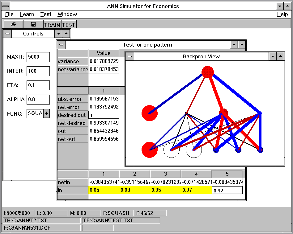
Figure 1: User interface of the simulator
The system consists of the following components:
- The runtime version of the APL interpreter. With this APL dialect the vendor allows distribution of the runtime interpreter version free of charge.
- The APL ANN workspace implements the classification system. The functions in the workspace are grouped into the following namespaces:
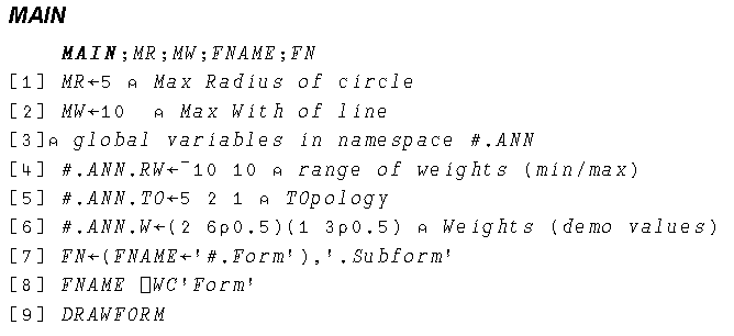
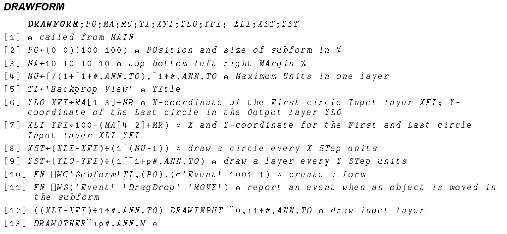
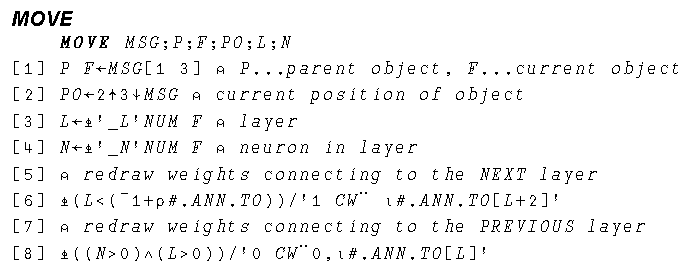
- Functions that create graphical objects like a window showing the multilayered perceptron network (see Figure 1). Often other than default properties are specified in GUI functions. Properties define an object's behavior, appearance and events that the object can generate. For each object able to generate events, a "callback function" can be assigned that is called when the corresponding event occurs. Events are very important for an application with a graphical front-end because they define how the objects react to the user. As an example, we show the APL code that allows the user to move the processing devices within the window.
- Functions for component file input and output. Because the execution time of such simulations is very high, logging facilities of the application must be provided. The application takes extensively advantage of nested vectors and matrices. With the component filesystem, APL variables can be created/appended directly to the hard disk.
- The last but not least part is the APL artificial neural network-code as described in [KR94]. The code consists of three individual parts: During network training, a main loop is used to present many input patterns to the artificial neural network. Within the loop there is a function that reads in and transforms the training data. The "FORWARD" function propagates the input pattern through the hidden layer(s) to the output layer. After the output value of the net is known, an error is calculated and the weight change is propagated backwards through the hidden layers to the input layer using the "BACKWARD" function.
The system is generally controlled via the graphical frontend because there is no session manager in the runtime version of the interpreter available.
Figure 1 shows the window of the "Multiple-Document Interface (MDI)" application. The MDI window consists of a menu bar and a tool bar at the top and a status field at the bottom. Within the main window, there are windows for general control of the system and for displaying details of the artificial neural network. The backprop view shows the activation level of the neurons (circles) and the weight values (lines). The window dump shows a net with 5 input, 3 hidden units and 1 output unit (5-3-1). A big filled circle indicates that the neuron fires and a transparent circle indicates (almost) no output of the neuron. The size of the circle is proportional to the output of a neuron. The lines connecting to each neuron from the previous layer are the graphical representation of the weight values. These can be negative or positive real numbers, which are encoded in two different colors. Again, a thick line represents a weight with a high negative or positive value.
Modeling
The Training Data
In order to indicate more practical relevance, we decided to use real data. First, we studied the insolvency statistics of the year 1993 [Hie93]:
- total amount of insolvencies: 5,082 (+38 %)
- total amount of obligations: US$ 2.9 Billion
- 17,000 employees evolved
In 1994, the "Atomic" company, one of the world's biggest producer of skiis became insolvent. Until now, the year 1994 seems to be another bad year of many insolvencies.
If we split up the total number of insolvencies according to types of company, we get the following statistics [Hie93]:
|
type of company |
percentage of total |
|
sole trader/partnership |
33.87 |
|
unlimited companies |
1.32 |
|
private limited companies |
50.66 |
|
public limited companies |
0.44 |
|
other |
13.71 |
Table 1: Which company types have a high risk to become insolvent?
Another important information is the membership of an individual company in the branch of industry. If we consider the branch of industry, the classification capability will probably be better. The metal-processing, paper, building and construction and the textile industry are the most jeopardized area of business in Austria.
After studying the possible sources of data about insolvent and sound companies, we decided to only survey private limited companies with a minimum turnover of US$ 30,000. Firstly private limited companies tend to become more often insolvent than other company types. Secondly private limited companies with more than ATS 1 Million common share or more than 300 employees have to publish their balance sheet.
What relationships between balance sheet items should be calculated to best describe the financial position of a business firm?
We decided to calculate the following five financial ratios to train our artificial neural network[Ble85]:
- cash flow / liabilities
- quick (current) assets / current liabilities
- quick (current) assets / total assets
- liabilities / total assets
- profit or loss / total assets
As test bed for our simulations we used 82 balance sheets, 59 of sound and 23 of insolvent companies. In order to average statistical outliers, we tried to get balance sheets of three successive years from each business firm. The 82 balance sheets were grouped in 62 training- and 20 test patterns.
The following figures show the distribution of the parameters:
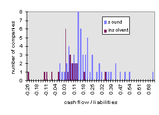
Figure 2: Distribution of balance sheet ratio cash flow / liabilities
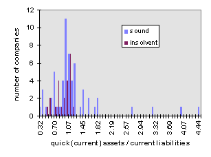
Figure 3: Distribution of balance sheet ratio quick (current) assets / current liabilities
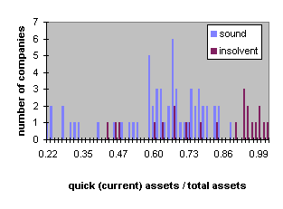
Figure 4: Distribution of balance sheet ratio quick (current) assets / total assets
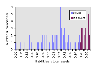
Figure 5: Distribution of balance sheet ratio liabilities / total assets
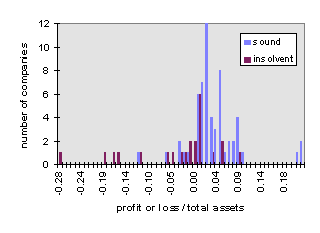
Figure 6: Distribution of balance sheet ratio profit or loss / total assets
The Algorithm
During the learning phase a randomly selected input/output pair is presented to the network. The input/output data is transformed into a range that the ANN can process. The output values are set to 1 for insolvent companies and to 0 for all others. The simulation environment helps the researcher to find a well performing network. Typically a session is divided into the following steps:
- Select a file for saving the network status in the file box menu
- Load the training data with the input/output pattern selection menu
- Set the network parameters (learning rate, momentum term, output function, maximum number of iterations) in the control menu
- Start learning
- Load test patterns and test the network
We have conducted many experiments to find the size of a well performing network. Table 2 and Figure 7 show the results of different network topologies in the test data sample after 5,000 learning iterations, using a learning rate of 0.3 and a momentum of 0.8.
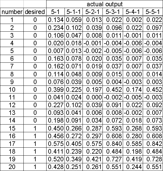
Table 2: Results for various network topologies
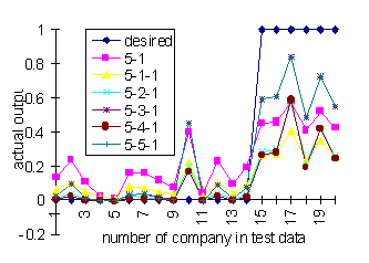
Figure 7: The performance of different network topologies
Because the network output has values between 0 and 1, we have to introduce a threshold to assign a company to the insolvent or sound cluster. For a threshold of 0.5, the 5-3-1 and 5-5-1 networks have the best performance with one wrong classification of an insolvent company (number 18).
We have chosen the smaller network for closer inspection.
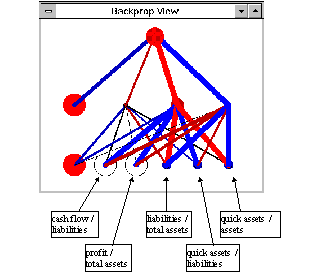
Figure 8: Graphical view of the found 5-3-1 network
The weight matrix between input (L0) and hidden (L1) layer is given in Table 3:

Table 3: The weight matrix between input and hidden layer
The weight vector between hidden (L1) and output (L2) layer is shown in Table 4:

Table 4: Weight vector between hidden and output layer
The Data was transformed with linear functions (see Table 5).

Table 5: Minimum and maximum values of original and transformed data
One neuron in the hidden layer is a detector for a sound and another for an insolvent company. The third neuron has a very small impact on the final result because of small weight values.
A company seems to be in danger when the ratio liabilities / total assets or quick assets / assets has a high positive value. On the other side, sound companies have small liabilities / total assets and quick assets / assets ratios.
Dyalog APL GUI Code
In this paper we want to present a piece of code, that implements the graphical user interface (GUI). The following functions implement the neuron (circles in figure) movable functionality. This enables the user to reposition the processing devices in the "backprop view" window. The circle is redrawn by APL itself. Only the weights (lines) connected to the neuron needs to repositioned. This is done with the function MOVE.




Conclusion
In this paper we have presented an APL tool for early detection of company failures using neural networks. This computing devices proved themselves to be a viable alternative to discriminant analysis.
With this workspace we were able to find networks for detection of company failures. Graphical visualization helps understanding complex relations that exist in neural nets.
Further work will include the improvement of the APL product and a detailed documentation of the user interface.
References
[Alf91] M. Alfonseca. Advanced applications of APL: logic programming, neural networks and hypertext. IBM Systems Journal, 30(4):543-553, 1991.
[Ble85] Ernst Bleier. Insolvenzfrüherkennung mittels praktischer Anwendung der Diskriminanzanalyse. Service Fachverlag an der Wirtschaftsuniversität Wien, Augasse 2-6, 1090 Vienna, Austria, 1985.
[Dya91] Dyadic Systems Limited, Riverside View, Basing Road, Old Basing, Basingstoke, Hampshire RG24 0AL, England. Dyalog Apl Users Guide for version 6.1, 1991.
[Dya94] Dyadic Systems Limited, Riverside View, Basing Road, Old Basing, Basingstoke, Hampshire RG24 0AL, England. Dyalog Apl User Guide, Language Reference, Windows Interface and Outer Products for Version 7.0, 1994.
[ES91] Richard M. Evans and Alvin J. Surkan. Relating Numbers of Processing Elements in a Sparse Distributed Memory Model to Learning Rate and Generalization. ACM APL Quote Quad, 21(4):166-173, 1991.
[GTBFS91] P. Gallinari, S. Thiria, F. Badran, and F. Folgelman-Soulie. On the Relations Between Discriminant Analysis and Multilayer Perceptrons. Neural Networks, 4:349-360, 1991.
[Hie93] Klaus Hierzenberger. Bericht zur Insovenzstatistik 1993. Kreditschutzverband von 1870, 1993.
[HKP91] John Hertz, Anders Krogh, and Richard G. Palmer. Introduction to the Theory od Neural Computation. Addison Wesley, Redwood City, California, 1991.
[HSW89] Kurt Hornik, Maxwell Stinchcombe, and Halbert White. Multilayer Feedforward Networks are Universal Approximators. Neural Networks, 2:359-366, 1989.
[KR94] Thomas Kolarik and Gottfried Rudorfer. Time Series Forecasting Using Neural Networks. ACM APL Quote Quad, 25(1):86-94, 1994.
[Nil90] Nils J. Nilsson. The Mathematical Foundations of Learning Machines. Morgan Kaufmann Publishers Inc., San Mateo, 1990.
[Pee81] Howard A. Peele. Teaching A Topic in Cybernetics with APL: An Introduction to Neural Net Modelling. ACM APL Quote Quad, 12(1):235-239, 1981.
[RHW86] David E. Rumelhart, Geoffrey E. Hinton, and Ronald J. Williams. Learning representations by backpropagating errors. Nature, 323(9):533-536, October 1986.
[RW94] Gottfried Rudorfer and Harald Wenisch. Isolvenzprognose mit Künstlichen Neuronalen Netzen. University of Economics and Business Administration, Augasse 2-6, 1090 Wienna, Austria, 1994.
[SS93] Alexei N. Skurihin and Alvin J. Surkan. Identification of Parallelism in Neural Networks by Simulation with Language J. ACM APL Quote Quad, 24(1):230-237, 1993.
[TK90] Kar Yan Tam and Melody Kiang. Predicting Bank Failures: A Neural Network Approach. Applied Artificial Intelligence, 4:265-282, 1990.


