")
")
Time Series Forecasting Using Neural Networks
Thomas Kolarik and Gottfried Rudorfer
Department of Applied Computer Science
Vienna University of Economics and Business Administration
Augasse 2-6, A-1090 Vienna, Austria
Diese E-Mail-Adresse ist vor Spambots geschützt! Zur Anzeige muss JavaScript eingeschaltet sein!
- Abstract
- Motivation
- A Very Short Introduction to Artificial Neural Networks
- Implementation
- Modeling
- Comparison with ARIMA Modeling
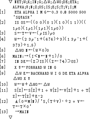
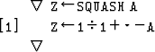
- Dyalog APL ANN Code
- Conclusion and Further Work
- References
- About this document ...
Abstract
Artificial neural networks are suitable for many tasks in pattern recognition and machine learning. In this paper we present an APL system for forecasting univariate time series with artificial neural networks. Unlike conventional techniques for time series analysis, an artificial neural network needs little information about the time series data and can be applied to a broad range of problems. However, the problem of network ``tuning'' remains: parameters of the backpropagation algorithm as well as the network topology need to be adjusted for optimal performance. For our application, we conducted experiments to find the right parameters for a forecasting network. The artificial neural networks that were found delivered a better forecasting performance than results obtained by the well known ARIMA technique.
Motivation
Time series analysis as described by most textbooks [Cha91] relies on explicit descriptive, stochastic, spectral or other models of processes that describe the real world phenomena generating the observed data.
Usually, the parameters of a standard model like the ARIMA technique [BJ76] are derived from the autocorrelation and frequency spectrum of the time series. Problems with the ARIMA approach arise with time series of increasing variance or when the time series represents nonlinear processes.
The usage of artificial neural networks for time series analysis relies purely on the data that were observed. As multi layer feed forward networks with at least one hidden layer and a sufficient number of hidden units are capable of approximating any measurable function [HSW89,SS91], an artificial neural network is powerful enough to represent any form of time series. The capability to generalize allows artificial neural networks to learn even in the case of noisy and/or missing data. Another advantage over linear models like the ARIMA technique is the network's ability to represent nonlinear time series.
The APL programming language is very suitable for the task of implementing neural networks [Alf91,Pee81,ES91,SS93] because of its ability of handle matrix and vector operations. The forward and backward paths of a fully connected feed forward network can be implemented by outer and inner products of vectors and matrices in a few lines of APL code.
For our application, we decided to use a fully connected, layered, feed forward artificial neural network with one hidden layer and the backpropagation learning algorithm. The next section gives a short overview of the relevant definitions and algorithms.
A Very Short Introduction to Artificial Neural Networks
As mentioned above, our simulations utilized the ``multi layered perceptron model'' (MLP), also known as ``feed forward networks'' trained with the ``generalized delta rule'', also known as ``backpropagation''.
The foundations of the backpropagation method for learning in neural networks were laid by [RHW86].
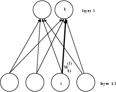
Artificial neural networks consist of many simple processing devices (called processing elements or neurons) grouped in layers. Each layer is identified by the index ![]() . The layers and L are called the ``input layer'' and ``output layer'', all other layers are called ``hidden layers''. The processing elements are interconnected as follows: Communication between processing elements is only allowed for processing elements of neighbouring layers. Neurons within a layer cannot communicate. Each neuron has a certain activation level a. The network processes data by the exchange of activation levels between connected neurons (see figure 1):
. The layers and L are called the ``input layer'' and ``output layer'', all other layers are called ``hidden layers''. The processing elements are interconnected as follows: Communication between processing elements is only allowed for processing elements of neighbouring layers. Neurons within a layer cannot communicate. Each neuron has a certain activation level a. The network processes data by the exchange of activation levels between connected neurons (see figure 1):
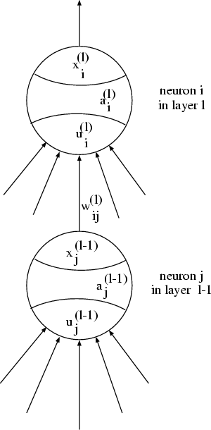
The output value of the i-th neuron in layer l is denoted by xi(l). It is calculated with the formula
xi(l) = g(ai(l))
where ![]() is a monotone increasing function. For our examples, we use the function
is a monotone increasing function. For our examples, we use the function ![]() (the ``squashing function''). The activation level ai(l) of the neuron i in layer l is calculated by
(the ``squashing function''). The activation level ai(l) of the neuron i in layer l is calculated by
ai(l) = f(ui(l))
where ![]() is the activation function (in our case the identity function is used).
is the activation function (in our case the identity function is used).
The net input ui(l) of neuron i in layer l is calculated as
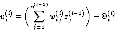
where wij(l) is the weight of neuron j in layer l-1 connected to neuron i in layer l, xj(l-1) is the output of neuron j in layer l-1. ![]() is a bias value that is subtracted from the sum of the weighted activations.
is a bias value that is subtracted from the sum of the weighted activations.
The calculation of the network status starts at the input layer and ends at the output layer. The input vector I initializes the activation levels of the neurons in the input layer:
![]()
For the input layer, ![]() is the identity function. The activation level of one layer is propagated to the next layer of the network. Then the weights between the neurons are changed by the backpropagation learning rule. The artificial neural network learns the input/output mapping by a stepwise change of the weights and minimizes the difference between the actual and desired output vector.
is the identity function. The activation level of one layer is propagated to the next layer of the network. Then the weights between the neurons are changed by the backpropagation learning rule. The artificial neural network learns the input/output mapping by a stepwise change of the weights and minimizes the difference between the actual and desired output vector.
The simulation can be divided into two main phases during network training: A randomly selected input/output pair is presented to the input layer of the network. The activation is then propagated to the hidden layers and finally to the output layer of the network.
In the next step the actual output vector is compared with the desired result. Error values are assigned to each neuron in the output layer. The error values are propagated back from the output layer to the hidden layers. The weights are changed so that there is a lower error for a new presentation of the same pattern. The so called ``generalized delta rule'' is used as learning procedure in multi layered perceptron networks.
The weight change in layer l at time v is calculated by
![]()
where ![]() is the learning rate and
is the learning rate and ![]() is the momentum. Both are kept constant during learning.
is the momentum. Both are kept constant during learning. ![]() is defined
is defined
- 1.
- for the output layer (l = L)
 as
as
where g'(ui(L)) is the gradient of the output function at ui(L).The gradient of the output function is always positive.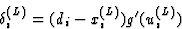
The formula can be explained as follows: When the output xk(l) of the neuron i in layer l is too small,
 has a negative value. Hence the output of the neuron can be raised by increasing the net input uk(l) by the following change of the weight values:
if xi(l-1) > 0, then increase wki(l)
if xi(l-1) < 0, then decrease wki(l)
The rule applies vice versa for a neuron with an output value that is too high (see figure 2).
- 2.
- for all neurons underneath the output layer (l < L)
 is defined by:
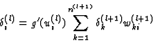
Finally the weights of layer l are adjusted by
![]()
Implementation
The time series modeling and forecasting system was implemented using Dyalog APL on HP 9000/700 workstations [Dya91] using the X11 window interface routines provided by the Xfns auxiliary processor. The system consists of two main components:
- A toolkit of APL functions that drive the neural network and log parameters and results of the simulation runs to APL component files.
- An X11-based graphical user interface that allows the user to navigate through the simulations and to compare the actual time series with the one generated by the neural network.
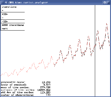
Figure 3 presents a screen dump![[*]](http://rudorfer.homedns.org/latex2html/foot_motif.gif) of the user interface: the broken line shows the actual time series, the solid line represents the network's output. The forecast data is separated from the historical data - the network's training set - by the vertical bar in the right quarter of the graph. The menu in the upper left corner of figure 3 allows the user to select a view of the network's forecasting capability at different states throughout the learning phase.
of the user interface: the broken line shows the actual time series, the solid line represents the network's output. The forecast data is separated from the historical data - the network's training set - by the vertical bar in the right quarter of the graph. The menu in the upper left corner of figure 3 allows the user to select a view of the network's forecasting capability at different states throughout the learning phase.
By browsing through the logfiles of the simulation runs, past and present results can be compared and analyzed.
 |
Modeling
The Training Sets
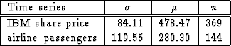
As test bed for our forecasting system we used two well known time series from [BJ76]: The monthly totals of international airline passengers (thousand of passengers) from 1949 to 1960 (see figure 4), and the daily closing prices of IBM common stock from May 1961 to November 1962 (see figure 5).
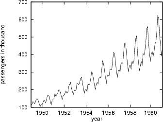
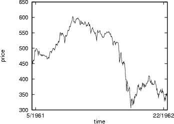
Table 1 gives some characteristics of these two time series: ![]() is the standard deviation,
is the standard deviation, ![]() the mean, and n the number of observations. The airline time series is an example of time series data with a clear trend and multiplicative seasonality, whereas the IBM share price shows a break in the last third of the series and no obvious trend and/or seasonality.
the mean, and n the number of observations. The airline time series is an example of time series data with a clear trend and multiplicative seasonality, whereas the IBM share price shows a break in the last third of the series and no obvious trend and/or seasonality.
The next section is concerned with the question: How can a neural network learn a time series?
The Algorithm
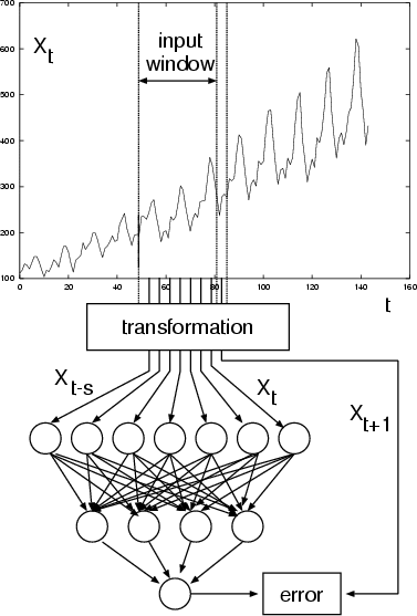
The neural network sees the time series ![]() in the form of many mappings of an input vector to an output value (see figure 6). This technique was presented by [CMMR92].
in the form of many mappings of an input vector to an output value (see figure 6). This technique was presented by [CMMR92].
A number of adjoining data points of the time series (the input window ![]() ) are mapped to the interval [0,1] and used as activation levels for the units of the input layer. The size s of the input window corresponds to the number of input units of the neural network. In a forward path, these activation levels are propagated over one hidden layer to one output unit. The error used for the backpropagation learning algorithm is now computed by comparing the value of the output unit with the transformed value of the time series at time t+1. This error is propagated back to the connections between output and hidden layer and to those between hidden and output layer. After all weights have been updated accordingly, one presentation has been completed. Training a neural network with the backpropagation algorithm usually requires that all representations of the input set (called one epoch) are presented many times. In our examples, we used 60 to 138 epochs.
) are mapped to the interval [0,1] and used as activation levels for the units of the input layer. The size s of the input window corresponds to the number of input units of the neural network. In a forward path, these activation levels are propagated over one hidden layer to one output unit. The error used for the backpropagation learning algorithm is now computed by comparing the value of the output unit with the transformed value of the time series at time t+1. This error is propagated back to the connections between output and hidden layer and to those between hidden and output layer. After all weights have been updated accordingly, one presentation has been completed. Training a neural network with the backpropagation algorithm usually requires that all representations of the input set (called one epoch) are presented many times. In our examples, we used 60 to 138 epochs.
For the learning of time series data, the representations were presented in a randomly manner: As reported by [CMMR92], choosing a random location for each representation's input window ensures better network performance and avoids local minima.
The next section is concerned with the selection of the right parameters for the learning algorithm and the selection of a suitable topology for the forecasting network.
Network Parameters
The following parameters of the artificial neural network were chosen for a closer inspection:
- The learning rate
 (
( ) is a scaling factor that tells the learning algorithm how strong the weights of the connections should be adjusted for a given error. A higher can be used to speed up the learning process, but if is too high, the algorithm will ``step over'' the optimum weights. The learning rate is constant across presentations.
 - The momentum

The momentum parameter
( ) is another number that affects the gradient descent of the weights: To prevent each connection from following every little change in the solution space immediately, the momentum term is added that keeps the direction of the previous step [HKP91], thus avoiding the descent into local minima. The momentum term is constant across presentations.
 - The number of input and the number of hidden units (the network topology).
The number of input units determines the number of periods the neural network ``looks into the past'' when predicting the future. The number of input units is equivalent to the size of the input window.
Whereas it has been shown that one hidden layer is sufficient to approximate continuous function [HSW89], the number of hidden units necessary is ``not known in general [HKP91]''. Other approaches for time series analysis with artificial neural networks report working network topologies (number of neurons in the input-hidden-output layer) of 8-8-1, 6-6-1 [CMMR92], and 5-5-1 [Whi88].
To examine the distribution of these parameters, we conducted a number of experiments: In subsequent runs of the network, these parameters were systematically changed to explore their effect on the network's modeling and forecasting capabilities.
We used the following terms to measure the modeling quality sm and forecasting quality sf of our system: For a time series ![]()
 |
(1) |
 |
(2) |
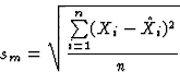
where ![]() is the estimate of the artificial neural network for period i and r is the number of forecasting periods. The error sm (equation 1) estimates the capability of the neural network to mimic the known data set, the error sf (equation 2) judges the networks's forecast capability for a forecast period of length r. In our experiments, we used r=20.
is the estimate of the artificial neural network for period i and r is the number of forecasting periods. The error sm (equation 1) estimates the capability of the neural network to mimic the known data set, the error sf (equation 2) judges the networks's forecast capability for a forecast period of length r. In our experiments, we used r=20.
Note: For reasons of clarity, in this section we only present graphics for the IBM share price time series. The graphics for the airline passenger time series are very similar.
The figures 7 and 8 demonstrate the effect of variations of the learning rate ![]() and the momentum
and the momentum ![]() on the modeling (figure 7) and forecast (figure 8) quality: both graphics give evidence for the robustness of the backpropagation algorithm, high values of both
on the modeling (figure 7) and forecast (figure 8) quality: both graphics give evidence for the robustness of the backpropagation algorithm, high values of both ![]() and
and ![]() should be avoided.
should be avoided.
![\begin{figure} \epsfxsize=80mm\epsfysize=80mm \centerline{ \epsfbox [0 247 595 842]{excel/reibmeaw.eps} }\end{figure}](http://rudorfer.homedns.org/apl94/img36.gif)
![\begin{figure} \epsfxsize=80mm\epsfysize=80mm \centerline{ \epsffile [0 247 595 842]{excel/reibmeap.eps} }\end{figure}](http://rudorfer.homedns.org/apl94/img37.gif)
The figures 10 and 11 present the effect of different network topologies on the modeling (figure 10) and forecasting (figure 11) quality: The number of input units and the number of hidden units open an interesting view: artificial neural networks with more than approx. 50 hidden units are not suited for the task of time series forecasting. This tendency of ``over-elaborate networks capable of data-miming'' is also reported by [Whi88].
Another parameter we have to consider is the number of presentations. A longer training period does not necessarily result in a better forecasting capability. Figure 9 demonstrates this ``overlearning'' effect for the IBM share price time series: with an increasing number of presentations, the network memorizes details of the time series data instead of learning its essential features. This loss of generalization power has a negative effect on the network's forecasting ability.
These estimations of the network's most important parameters, although rough, allowed us to choose reasonable parameters for our performance comparison with the ARIMA technique, described in the next section.
![\begin{figure} \epsfxsize=80mm\epsfysize=80mm \centerline{ \epsffile [0 247 595 842]{excel/reibmihw.eps} }\end{figure}](http://rudorfer.homedns.org/apl94/img39.gif)
|
Comparison with ARIMA ModelingWe compared our results with the results of the ARIMA procedure of the SAS software, an integrated system for data access, management, analysis and presentation. The implementation of the ARIMA procedure of SAS follows the programs described by Box and Jenkins in Part V of their classic [BJ76]. The ARIMA model is called an autoregressive integrated moving average process of order (p, d, q). It is described by the equation
We fitted an ARIMA model for each time series using the SAS system and let it predict the next 20 observations of the time series. The last 20 observations were dropped from the time series and used to calculate the prediction error of the models. The following ARIMA models were calculated for the airline passenger time series (after a logarithmic transformation): (1-z)(1-z12)Xt = (1 - 0.24169z - 0.47962z12) Ut and for the IBM time series:(1-z) Xt = (1 - 0.10538z) Ut As an opponent for the ARIMA modeling technique, we selected those networks that delivered the smallest forecast error sf for the respective time series data:
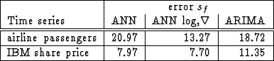
In Table 2 the prediction errors for the artificial neural network (ANN), the artificial neural network using the logarithmic and
|
![\begin{figure} \epsfxsize=80mm\epsfysize=80mm \centerline{ \epsffile [0 247 595 842]{excel/reibmihp.eps} }\end{figure}](http://rudorfer.homedns.org/apl94/img40.gif)